Objectives
- Determine intrinsic viscosities for a polymer-solvent system.
- Determine Mark-Houwink "K" and "a" values for a polymer-solvent system.
- Determine molecular weight of an unknown polymer using "K" and "a" values.
Introduction
All polymers increase the viscosity of the solvent in which they are dissolved. This increase allows for a convenient method of determining the molecular weight of polymers. Since the viscosity method is not based on rigorous physical laws, it must be calibrated by standards of known molecular weight with narrow molecular weight distributions.
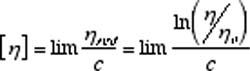
Several important viscosity functions are used in viscosity studies. The relative viscosity, hr = h / h o , is the dimensionless ratio of solution viscosity, h, to solvent viscosity, h o. The specific viscosity, h sp = (h - h o) /h o , is related to the fluid viscosity increase due to all polymer solute molecules. The reduced viscosity, h red = h sp /c , is the fluid viscosity increase per unit of polymer solute concentration, c. The intrinsic viscosity, [h] is the limit of the reduced viscosity as the polymer solute concentration approaches zero. The intrinsic viscosity is also the limit of the inherent viscosity, ln(h / h o), as the solution polymer concentration approaches zero.
Extrapolation to zero polymer concentration is intended to eliminate polymer intermolecular interactions. When the polymer concentration is expressed in g/dl, the units of [h] will be dl/g. The plots used to find the intrinsic viscosity are called the Huggins plot ( h red vs. c ) and the Kraemer plot ( ln(h / ho) vs. c ). As shown in Figure 1, the curves of both plots should be linear and have a common intercept that is the intrinsic viscosity.

Figure 1 : Typical Huggins and Kraemer Plots (note common intercept for both curves)
The intrinsic viscosity (also termed the limiting viscosity number) should be independent of the fluid shear rate. In other words, the solution viscosities measured and used to find the intrinsic viscosity in the Huggins or Kraemer plots must be the "zero" shear viscosities determined in the low shear or first Newtonian regions of flow curves. A flow curve is a plot of apparent fluid viscosities versus shear rate. Each flow curve is experimentally determined using a fixed polymer concentration. If the polymer solution concentrations are low and the polymer molecular weights are also low, then the solution viscosities measured for the flow curve are constant or independent of the shear rate. The solution viscosities measured under these conditions are first Newtonian viscosities or the “zero” shear viscosities. However, as the polymer concentration increases and/or the polymer molecular weigh increases, the flow curves become shear dependent or non-Newtonian. Usually, for non-Newtonian polymer solutions the apparent solution viscosity decreases as the shear rate increases. This type fluid is usually referred to as shear thinning or pseudoplastic fluid flow behavior. See Figure 2. To minimize the unwanted shear thinning effect, it is desirable to operate a viscometer at low shear rates.
Figure 2: Typical Flow Curve (note that as the molecular weight decreases, shear thinning behavior starts at greater shear rates)
From polymer dilute solution viscosity experiments, many macromolecular characteristics of a polymer can be determined such as molecular weight and certain polymer hydrodynamic dimensions. These experiments are not time consuming and do not require expensive equipment.
The intrinsic viscosity measured in a specific solvent is related to the molecular weight, M, by the Mark-Houwink equation.
[h] = K Ma
where K and a are Mark-Houwink constants that depend upon the type of polymer, solvent, and the temperature of the viscosity determinations. The exponent ‘a ’ is a function of polymer geometry, and varies from 0.5 to 2.0. These constants can be determined experimentally by measuring the intrinsic viscosities of several polymer samples for which the molecular weight has been determined by an independent method (i.e. osmotic pressure or light scattering). Using the polymer standards, a plot of the log [h] vs log M usually gives a straight line. The slope of this line is the "a" value and the intercept is equal to the log of the "K" value. See Figure 3.
Figure 3: Typical Mark-Houwink Plot (note that the fit line slope is the ‘a’ value)
The fact that the intrinsic viscosity of a given polymer sample is different in different solvents gives one insight into the general shape of polymer molecules in solution. A long-chain polymer molecule in solution takes on a somewhat kinked or curled shape, intermediate between a tightly curled mass (coil) and a rigid linear configuration. All possible degrees of curling may be displayed by any one molecule, but there will be an average configuration which will depend on the solvent. In a “good” solvent, one that shows a zero or negative heat of mixing with the polymer, the molecule is fairly loosely extended, and the intrinsic viscosity is high. The Mark-Houwink "a" constant is close to 0.75 or higher for these "good" solvents. In a "poor" solvent, one that shows a positive heat of mixing, segments of a polymer moleculeattract each other in solution more strongly than they attract surrounding solvent molecules. The polymer molecule assumes a tighter configuration, and the solution has a lower intrinsic viscosity. The Mark-Houwink "a" constant is close to 0.5 in "poor" solvents. For a rigid or rod like polymer molecule that is greatly extended in solution, the Mark-Houwink ‘a’ constant approaches a value of 2.0.
This experiment allows students to carry out classic capillary viscosity experiments on polymer standards to determine Mark-Houwink constants. These constants are then used to determine the viscous average molecular weight of an unknown polymer.
Experimental
- Select one of the aqueous polyethylene oxide (PEO) solutions provided. Several solutions have been made using different polymer molecular weights and at different concentrations. Record the specifications of the polymer solution you selected.
- Pour into a working cup about 25 mL of the selected polymer solution. Use this fluid to make the viscosity measurements explained below.
- Cannon-Fenske Operating Instructions: (See Figure 4 and Table I)
- Select a Cannon-Fenske viscometer that will give a efflux flow time greater than 200 sec or the minimum time specified in Table I, shown below. The MathCad worksheet "PEO_Solution_Viscosities.mcd" can be used to help determine the appropriate viscometer size. See Appendix A. You will utilize a No. 25 size Cannon-Fenske viscometer for all solutions used this experiment. Clean the viscometer with suitable solvents (water and acetone) and blow dry, clean, filtered nitrogen gas through viscometer to remove all traces of solvent.
- Introduce the fluid sample from the working cup into the viscometer by pipetting 10 ml into Tube L.
- Place the viscometer in a constant-temperature bath. Mount the viscometer upright in the bath keeping Tube L vertical. Allow time (about 15 minutes) for the sample fluid to attain bath temperature and become free of air bubbles.
- Apply suction to Tube N or pressure to Tube L to force the fluid sample into Bulb D about 2 cm above upper timing Mark E.
- Remove the pressure or vacuum and allow the fluid sample to flow down through Capillary R by the force of gravity. Measure the efflux time, to the nearest 0.1 second, required for the leading edge of the fluid meniscus to pass from timing Mark E to timing Mark F. If the efflux time is less than the minimum (250 sec for the No 25 viscometer), select a smaller size capillary viscometer and repeat steps a through e.
- Repeat steps d and e making at least three measurements of the fluid efflux time. The reading should agree to within 0.1% of the average flow time. If flow time variation is noted, repeat efflux time measurement six times and take the average of three readings that are within 0.1% of each other. Record the efflux times. Recall that a fluid’s efflux flow time is proportional to the fluid’s viscosity.
- Repeat steps 1 through 3 for four solution concentrations having a constant polymer molecular weight.
- Repeat steps 1 through 4 for a second set of molecular weight polymer standard solutions.
- Repeat steps 1 through 4 for the unknown molecular weight polymer solutions.
- Repeat step 3 using only the solvent (water). The efflux time for water is proportional to the water’s viscosity at the temperature of the measurement. At 20.2oC the viscosity of water is 1.0000 centipoise, at 23oC the viscosity is 0.9358 centipoise, and at 25oC the viscosity is 0.8937 centipoise.
| Table I: Properties of Cannon-Fenske Viscometers (see Figure 4) | ||||||
|---|---|---|---|---|---|---|
| Size No. | Approximate Constant, cSt/s | Kinematic Viscosity Range, cSt | Inside Diameter of Tube R, mm(+2%) | Inside Diameter of Tubes N, E, and P, mm | Bulb Volume, ml (5%) | |
| 25 | 0.002 | 0.5A to 2 | 0.30 | 2.6 to 3.0 | 3.1 | 1.6 |
| 50 | 0.004 | 0.8 to 4 | 0.44 | 2.6 to 3.0 | 3.1 | 3.1 |
| 75 | 0.008 | 1.6 to 8 | 0.54 | 2.6 to 3.2 | 3.1 | 3.1 |
| 100 | 0.015 | 3 to 15 | 0.63 | 2.8 to 3.6 | 3.1 | 3.1 |
| 150 | 0.035 | 7 to 35 | 0.78 | 2.8 to 3.6 | 3.1 | 3.1 |
| 200 | 0.1 | 20 to 100 | 1.01 | 2.8 to 3.6 | 3.1 | 3.1 |
| 300 | 0.25 | 50 to 250 | 1.27 | 2.8 to 3.6 | 3.1 | 3.1 |
| 350 | 0.5 | 100 to 500 | 1.52 | 3.0 to 3.8 | 3.1 | 3.1 |
| 400 | 1.2 | 240 to 1200 | 1.92 | 3.0 to 3.8 | 3.1 | 3.1 |
| 450 | 2.5 | 500 to 2500 | 2.35 | 3.5 to 4.2 | 3.1 | 3.1 |
| 500 | 8 | 1600 to 8000 | 3.20 | 3.7 to 4.2 | 3.1 | 3.1 |
| 600 | 20 | 4000 to 200000 | 4.20 | 4.4 to 5.0 | 4.3 | 3.1 |
| A 250-s minimum flow time for all other units. | ||||||
Calculations
Make a table of concentration (g/100 ml), efflux time (sec.), h / h0, h sp / c, and ln(h r / c).
For each molecular weight polymer standard, plot h sp /c vs. c and ln(hr /c) on the same plot. Thereafter use each plot to determine the intrinsic viscosity of each polymer standard.
Using the intrinsic viscosities and the corresponding polymer molecular weights, plot log [h] vs. log MW and then use this plot to determine the Mark-Houwink ‘K’ and ‘a’ constants for the polyethylene-water system.
Finally, calculate the molecular weight of the unknown PEO from the Mark-Houwink equation and the intrinsic viscosity of the unknown.
Discussion
Compare your polyethylene-water calculated 5 and a values with reported literature values (See Polymer Handbook ).
Discuss the effect of a variation in fluid temperature on solution viscosity from a molecular viewpoint.
From a molecular viewpoint, discuss the solution viscosity differences you would expect in a good solvent versus using a poor solvent.
Discuss any experimental error associated with measuring the solution viscosities. Do you have any suggestions that would reduce experimental error or simplify the experimentation?
Discuss your estimate of the molecular weight of the unknown PEO sample. What quantitative confidence interval would you report for the molecular weight value you estimated for the unknown PEO ?
 Return to
Macrolab Directory
Return to
Macrolab Directory